Material in Unit 6 is optional. You are not expected to know this for a test and there are no labs or projects using this material.
Introduction to pandas
This guide shows you the basics of using pandas to plot data.
If you are writing code on your own machine, be sure to install pandas first:
pip install pandasYou can view a Google Colab notebook of this guide page.
Reading a CSV file into a dataframe
One of the nicest things about pandas is you can read data from a CSV file. In fact, you can read files directly over the Internet by providing a URL for the file.
data = pd.read_csv(filename_or_URL)The result of reading the CSV is a dataframe, which is a two-dimension representation of your data — just like a spreadsheet.
You can take a look at the first few lines of the dataframe using data.head().
import pandas as pd

world_pop = pd.read_csv("https://raw.githubusercontent.com/zappala/intro-to-pandas/main/world-population.csv")
print(world_pop.head())
This will show the first five rows of the dataframe:
   LocID Location  VarID  ...    PopFemale     PopTotal  PopDensity
0    900    World      2  ...  1270171.462  2536431.018      19.497
1    900    World      2  ...  1293796.589  2584034.227      19.863
2    900    World      2  ...  1317007.125  2630861.690      20.223
3    900    World      2  ...  1340156.275  2677609.061      20.582
4    900    World      2  ...  1363532.920  2724846.754      20.945

[5 rows x 10 columns]
This data comes from a collection of world population data provided by the United Nations. It’s a really large file, with separate data for every country from 1950 onward, so I have created a smaller set of it that provides just the population data for the entire world.
You can look at the last few lines of the data with:
print(data.tail())This will show the last five rows of the datframe:
     LocID Location  VarID  ...    PopFemale      PopTotal  PopDensity
146    900    World      2  ...  5418979.294  1.085811e+07      83.464
147    900    World      2  ...  5422249.024  1.086361e+07      83.506
148    900    World      2  ...  5425118.647  1.086835e+07      83.542
149    900    World      2  ...  5427571.318  1.087228e+07      83.573
150    900    World      2  ...  5429588.256  1.087539e+07      83.596

[5 rows x 10 columns]
Notice that the data goes to the year 2100! All the data after the current year is a projection.
Getting columns of the dataframe
You can get a single column of the dataframe by putting the name of the column in square brackets:
print(world_pop['PopTotal'])This will print:
0      2.536431e+06
1      2.584034e+06
2      2.630862e+06
3      2.677609e+06
4      2.724847e+06
           ...
146    1.085811e+07
147    1.086361e+07
148    1.086835e+07
149    1.087228e+07
150    1.087539e+07
Name: PopTotal, Length: 151, dtype: float64
You can also get multiple columns from the dataframe:
print(world_pop[['Time', 'PopTotal', 'PopMale', 'PopFemale']])This will print:
     Time      PopTotal      PopMale    PopFemale
0    1950  2.536431e+06  1266259.556  1270171.462
1    1951  2.584034e+06  1290237.638  1293796.589
2    1952  2.630862e+06  1313854.565  1317007.125
3    1953  2.677609e+06  1337452.786  1340156.275
4    1954  2.724847e+06  1361313.834  1363532.920
..    ...           ...          ...          ...
146  2096  1.085811e+07  5439132.293  5418979.294
147  2097  1.086361e+07  5441365.752  5422249.024
148  2098  1.086835e+07  5443228.989  5425118.647
149  2099  1.087228e+07  5444712.816  5427571.318
150  2100  1.087539e+07  5445805.463  5429588.256

[151 rows x 4 columns]
Keep in mind that these return a new copy of the dataframe. The original is unchanged. So if you want to keep that copy, you need to store it in a variable.
total_population = world_pop[['Time', 'PopTotal']]
print(total_population.head())
This prints:
   Time     PopTotal
0  1950  2536431.018
1  1951  2584034.227
2  1952  2630861.690
3  1953  2677609.061
4  1954  2724846.754
Using specific rows from the dataframe
You can get specific rows from the data frame by putting the row number in square brackets:
print(world_pop.loc[1])This prints:
LocID                 900
Location            World
VarID                   2
Variant            Medium
Time                 1951
MidPeriod          1951.5
PopMale       1290237.638
PopFemale     1293796.589
PopTotal      2584034.227
PopDensity         19.863
Name: 1, dtype: object
You can get a set of rows and their columns by listing a range of rows and a set of columns:
print(world_pop.loc[1:10, ['Time', 'PopTotal']])This prints:
    Time     PopTotal
1   1951  2584034.227
2   1952  2630861.690
3   1953  2677609.061
4   1954  2724846.754
5   1955  2773019.915
6   1956  2822443.254
7   1957  2873306.058
8   1958  2925686.680
9   1959  2979576.147
10  1960  3034949.715
You can get all the rows by using just ’:’ for the row specifier:
print(world_pop.loc[:, ['Time', 'PopTotal']])This prints:
     Time      PopTotal
0    1950  2.536431e+06
1    1951  2.584034e+06
2    1952  2.630862e+06
3    1953  2.677609e+06
4    1954  2.724847e+06
..    ...           ...
146  2096  1.085811e+07
147  2097  1.086361e+07
148  2098  1.086835e+07
149  2099  1.087228e+07
150  2100  1.087539e+07

[151 rows x 2 columns]
You can get a subset of rows by using boolean conditions:
print(world_pop.loc[(world_pop['Time'] >= 2010) & (world_pop['Time'] <= 2020), ['Time','PopTotal']])This prints:
Time PopTotal
60 2010 6956823.588
61 2011 7041194.168
62 2012 7125827.957
63 2013 7210582.041
64 2014 7295290.759
65 2015 7379796.967
66 2016 7464021.934
67 2017 7547858.900
68 2018 7631091.113
69 2019 7713468.205
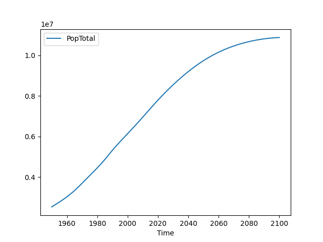
70 2020 7794798.729Plotting a dataframe
Pandas makes it really easy to create plots from the data in a dataframe. Here is a simple line plot of the total population by year:
world_pop.plot(x='Time', y='PopTotal')This produces a plot:
If you want to save this to a file:
ax = world_pop.plot(x='Time', y='PopTotal')
figure = ax.get_figure()
figure.savefig('population.png')
We can plot multiple lines at a time by providing multiple y values in a list:
world_pop.plot(x="Time", y=["PopMale","PopFemale","PopTotal"])This produces a plot:
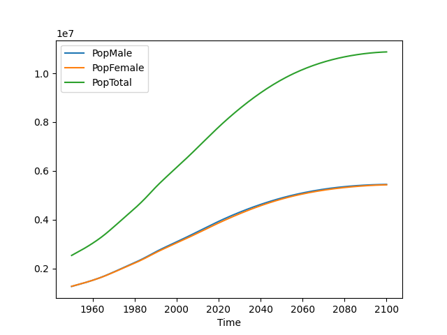
Note that the male and female populations are nearly identical.
Sometimes we need to chain together multiple plots, and we can do that with the
axis returned by the plot() function:
ax = world_pop.plot(x="Time", y="PopMale")
world_pop.plot(ax = ax, x="Time", y="PopFemale")
world_pop.plot(ax = ax, x="Time", y="PopTotal")
This produces the same plot as above.
Creating new columns
It can be useful to create new columns in the dataframe. Here we create a new column that converts the population in thousands to the billions.
world_pop["PopTotalBillions"] = world_pop["PopTotal"] / 1e6
print(world_pop.head())
This prints:
LocID Location VarID ... PopTotal PopDensity PopTotalBillions
0 900 World 2 ... 2536431.018 19.497 2.536431
1 900 World 2 ... 2584034.227 19.863 2.584034
2 900 World 2 ... 2630861.690 20.223 2.630862
3 900 World 2 ... 2677609.061 20.582 2.677609
4 900 World 2 ... 2724846.754 20.945 2.724847
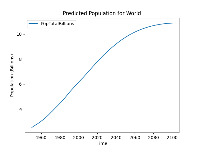
[5 rows x 11 columns]Adding labels to plots
We can specify additional parameters to plot() to modify the x labels, y
labels, and title.
world_pop.plot(
    x='Time',
    y="PopTotalBillions",
    ylabel="Population (Billions)",
    title="Predicted Population for World"
)
This creates the plot: